Interactive Computational Fluid Dynamics Solver
Dr. Clarence Burg and Mark VanderLugt
Previous efforts by Ethan Hereth,
Dane Womack and Taylor Erwin
The goal of this project, supported by an internal grant from the University of Central Arkansas’ University Research Council, was to develop a interactive platform for computational fluid dynamics simulations that would be appropriate for high school science courses and science museum exhibits. The original efforts in 2008 resulted in three distinct codes - a graphical user interface for specifying the solver options and flow conditions, a visualizer for the solution and the computational fluid dynamics solver. In the 2010-2011 academic year, Mark VanderLugt used his Java skills to combine the three codes into a single code, building upon the original efforts, streamlining the user interface, improving the visualization options and integrating the CFD solver seamlessly within the Java program.
Computational Fluid Dynamics involves the modeling of fluid flows, such as air and water, around objects of interest to scientists and engineers. Using physical laws such as the conservation of mass, momentum and energy and developing physical models for friction, complicated mathematical equations are derived, which can only be solved approximately using computational tools. Hence, computational fluid dynamics is a highly interdisciplinary field, combining physics and fluid dynamics with mathematics and computer science in the context of science and engineering investigations. Applications of computational fluid dynamics include:
· Flight and aerospace engineering – the flow of air around planes and missiles and the combustion of fuel in engines and rockets
· Oil and gas exploration, along with underground water flows
· Weather prediction and atmospheric modeling, including storms, hurricanes and tornados
· Modeling of planetary atmospheres and of solar events through a better understanding of the solar atmosphere
· Pipe flows, for oil pipelines and for water and sewage transport within cities
The process of computational fluid dynamics typically involves the following steps:
· Building the geometry on a computer – the shape of the wing, the size and dimensions of the underground reservoir, the length, diameter and connections of pipes within a network, etc.
· Generation of a mesh or grid where the fluid (air or water) flows – around a wing, inside the pipe, etc.
· Specification of flow parameters and boundary conditions – how fast is the air or water flowing, what is the pressure, what is the density and viscosity of the fluid?
· Calculation of the flow using a computational fluid dynamics solver on the mesh under the specified flow conditions
· Visualization and analysis of the computational results
Interactive CFD Program
There are two difference CFD solvers – the compressible version (i.e., air) and the incompressible version (i.e., water). They can be downloaded at
http://faculty.uca.edu/clarenceb/Compressible_CFD_UCA.zip
http://faculty.uca.edu/clarenceb/Incompressible_CFD_UCA.zip
You will need to unzip the file by extracting the contents (After downloading the file, move the file to an appropriate location, right click on the file and select ‘Extract All’)
The contents consist of the executable file InteractiveCFD.jnlp and three directories, containing the Cases, the JavaResource and the Solver. The Cases directory contains the various grids for the air flow simulations, the JavaResources contains third-party Java executables that are used by the InteractiveCFD executable and the Solver directory contains the two Java codes that control the user interface and the CFD solver.
To run the Interactive CFD solver, click on the file InteractiveCFD.jnlp. The program will automatically load and display the first case in the Surf Reader listing. You can select a different case by scrolling through the list of cases. Once selected, the program will automatically load and display that geometry and grid. You can select the Mach number and the angle of attack, as well as the Reynolds number. Once these are chosen, click RUN to begin the simulation. You can change these values during the simulation.
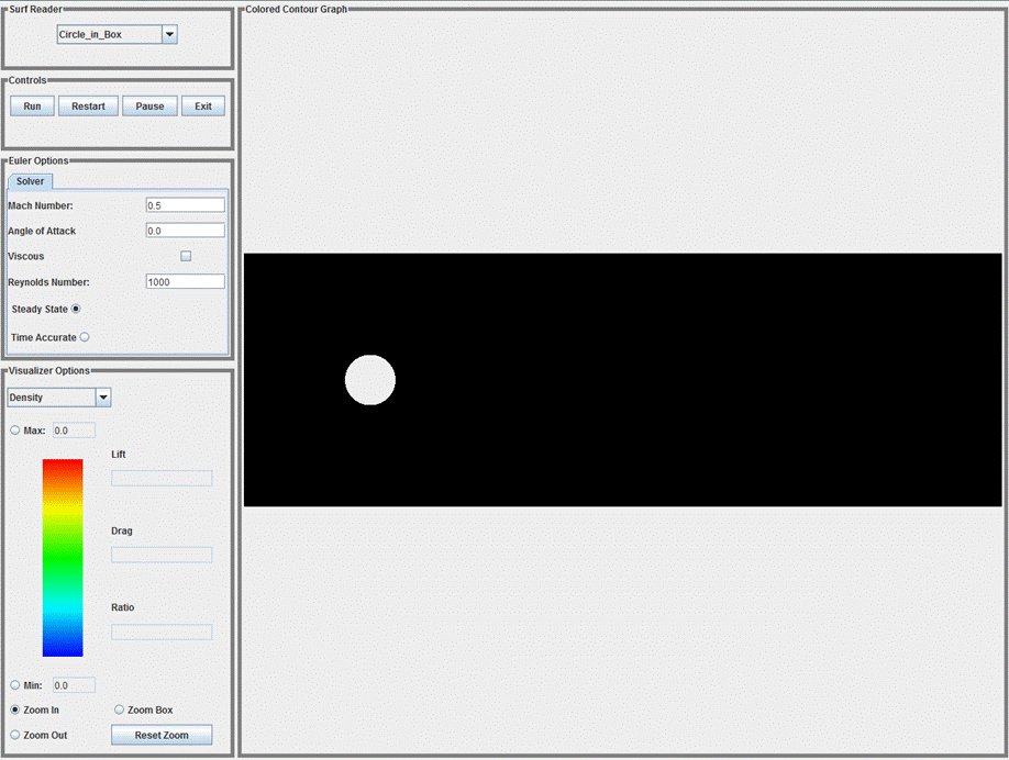
The visualizer shows the current solution variable, such as the density, pressure, x-velocity and Mach number. Red and white are high values while blue and black are low values. The maximum and minimum values are calculated each time that the solution is displayed, but these values can be user defined as well. The lift and drag coefficients are calculated for the solid surfaces, as well as the lift to drag ratio. The user can also zoom in and out of the visualization window.
Solver and Visualizer Options
For air flow, the Mach number is the ratio of the air speed to the speed of sound in air. Thus, Mach 1 represents the speed of sound, which is approximately 750 mph at sea level. Mach 0.5 represents half of the speed of sound and is in the subsonic range. Values of Mach that are greater than 1 are supersonic. Air flow characteristics change significantly between subsonic and supersonic flows.
The angle of attack is the angle between the primary axis of the geometry and the air flow direction. Typically, angle 0 indicates that the geometry is pointing directly into the wind. A positive angle of attack means that the air flow is approaching the geometry from below, while a negative angle of attack means that the air is blowing downwards onto the geometry.
The Reynolds number is a measure of the viscosity or friction within the simulation. It is the ratio of inertia forces to the viscous forces, which can be interpreted as the ratio of the strength of the air flow to resistance generated by friction. A higher Reynolds number indicates a low amount of friction. For these simulations, the Reynolds number must be greater than or equal to 1000. The viscous box must be checked for the Reynolds number to have any impact on the simulation.
The Steady State and the Time Accurate options control the influence of the changes in time on the simulation. Due to the manner in which time evolution is handled within the solver, these options have little impact on the simulation.
For the visualizer options, the user can select the variable to be displayed, including density, pressure, x and y velocity components, the local Mach number in the flow which is just the magnitude of the local velocity, and the energy. The maximum and minimum values are displayed on the color bar for the color legend, unless the user specifies these values.
The user can zoom in, zoom out or zoom in on a box within the simulation.
The lift coefficient and drag coefficient calculate the pressure drag on the solid surfaces. The lift coefficient is calculated based on the pressure component in the vertical direction, while the drag coefficient is calculated based on the pressure component in the horizontal direction. The lift to drag ratio is the ratio of these two components. For a wing to support an airplane, it must have positive lift. The higher the lift to drag ratio the more efficient the wing is at the specified Mach and Reynolds number.
Geometries/Cases
Several geometries or cases have been built and included within the Interactive_CFD_UCA.zip file. If the case ends in _v, then the solid walls have a viscous boundary condition imposed, which means that the velocity along the wall is approximately 0; otherwise the velocity is parallel to the solid wall.
Several of the geometries have the name NACA followed by 4 numbers. These were generated based on formula developed by the National Advisory Committee on Aeronautics based on the 4 digits series and determine the camber, the camber location and the maximum thickness of the wing. Hence, the NACA 2412 airfoil has a camber of 2% located 40% from the leading edge to the trailing edge with a thickness of 12% over the length of the airfoil.
A wide variety of NACA 4 digit wings can quickly generated upon request. Other types of geometries can be also built. Please send ideas for additional geometries to clarenceb@uca.edu
The grid format is quite simple for an unstructured triangular and quadrilateral meshes. It is described below:
Number_Of_Triangles Number_of_Quadrilaterals Number_of_Nodes
x y z locations for each node (there are Number_of_Nodes of these triplets)
n0 n1 n2 node numbers for each triangle (there are Number_of_Triangles of these triplets)
n0 n1 n2 n3 node numbers for each quadrilateral (there are Number_of_Quadrilaterals of these sets)
Number_of_Boundary_Edges
n0 n1 boundary_number (there are Number_of_Boundary_Edges of these sets)
Number_of_Boundary_Types
Type Name (there are are Number_of_Boundary_Types of these sets)
Boundary types include:
0 – empty
1 – outer boundary (flow through)
2 – solid wall (inviscid, velocity parallel to wall)
3 – viscous wall (velocity approximately 0)
You can build your own grids and place in the cases directory. The InteractiveCFD solver should automatically detect these new cases.
Please send suggestions and comments to clarenceb@uca.edu