PHYS 1401: Descriptive Astronomy

Introduction

Since the first extra-solar planet was discovered in 1989, there have been over 1000 additional planets confirmed to be orbiting other suns. In the fall of 1995, astronomers were excited by the possibility of a planet orbiting a star in the constellation Pegasus. Why such a fuss over this particular star (called 51 Pegasi), located 50 light years from the Earth? Because it is a star almost identical to our own sun! Just slightly more massive and a bit cooler than the Sun, it seemed like a good place to look for planets−given that we know for a fact that at least one sun-like star (our own!) has an extensive planetary system, with at least one planet (our own!) capable of supporting life!

Objectives

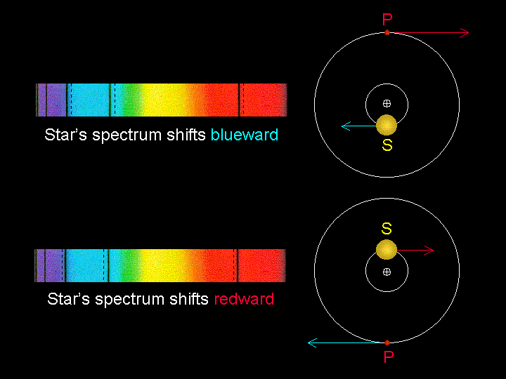
• Identify the presence of an extra-solar planet by its effect on its parent star
• Prepare an accurately scaled graph of radial velocity data
• Perform basic curve fitting to match plotted data
• Calculate the orbital period of the exoplanet and use it to locate the planet's distance from its star
• Determine the mass of this newly discovered exoplanet

Procedure

Until very recently, the most common method of exoplanet detection involves radial velocity measurements. As we know, the light from an object moving towards us will be shifted toward shorter wavelengths (blue-shifted), and motion away results in light that is red-shifted towards longer wavelengths. This Doppler shift can be used to calculate the speed with which an object is hurtling at us through space.

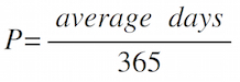
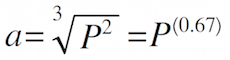
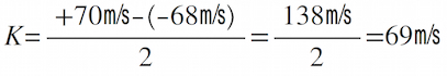
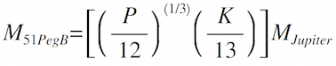
Well, how does this help us "see" a very tiny planet orbiting a very distant star? Even if the planet is too small for us to image directly, its presence can be detected by its gravitational pull on the star it orbits. Technically, the star and planet are both orbiting their common center of mass. Because the star is so much larger, the planet moves very noticeably, and the star remains virtually stationary. But it's not quite perfectly still: the star will wobble slightly with each orbit of the planet, first one way, then the other. Since the planet's orbit is periodic (Kepler! Number! Three!), so is the wobble of the parent star. What that means is that the star's radial velocity will change slightly, increasing and decreasing with the same periodicity as the planet's orbit.

With each orbit of the planet, you can watch any particular spectral line you like (maybe the H_α?) shift slightly to the red, then to the blue. Because you know where the line ought to be (656nm), you can determine the radial velocity, and the bigger the Doppler shift, the more massive the planet is. The period of the planet in orbit can be measured by watching the pattern repeat. And once you know there's a planet out there, and what its orbit looks like, it's not that hard to calculate its mass (Newtonian Gravity and Kepler #3!).

Data & Analysis

The table below is some of the actual Marcy & Butler data collected in October of 1995 at the Lick Observatory in California.

1. Graph the data: Plot the above data in your lab notebook. Scale the time in days on the x-axis, and the radial velocity on the y-axis. It is very important that you scale your axes accurately and consistently. On the time axis (x), run from 0 to 14 days, and on the velocity axis (y) scale from −70 to +70 m/s.

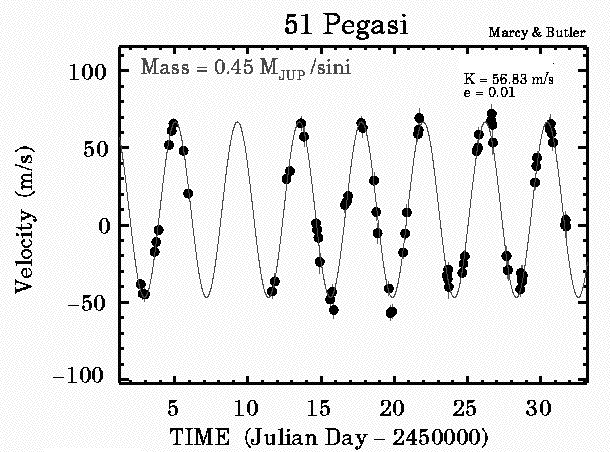
Your graph will not be identical to this one! However, it should give you an idea of what to expect as you plot your own data.

2. Fit the curve: Once you have the points plotted, carefully sketch a curve fit. The shape should be a sine curve, like you see above. Notice above that, even if there are gaps in the data, the curve is smooth and continuous.

Questions

1. Why sine? Why is a sine curve used to fit this data? Why not just connect the dots?
2. Why are there gaps in this data set? Look at the pattern, and notice two reasons for missing data. How could you compensate for this?
3. Determine the orbital period of the planet: There are several methods to extract this information from your graph. Use at least two different techniques to obtain at least three separate values, then calculate the average period in days.
4. Convert the average period in days to years:



5. Find the distance: Use the average period P in years and Kepler #3 to calculate the average distance a (in AU) of the planet from its star:



6. Average the amplitude: Examine your graph again, and record the maximum (+) and (−) amplitudes of the sine curve. For example, if the maximum (+) velocity is +70, and the maximum (−) velocity is −68, then the amplitude K is:


(Note: Your value is not going to be exactly 69m/s!)

7. Calculate the mass: By combining Kepler #3 with Newton's Universal Gravitation, we can calculate the mass of 51 Pegasi b. Instead of an absolute mass in kilograms, we will calculate based on comparison to Jupiter. Once we have combined Kepler and Newton, then performed the unit conversions we are left with: where P and K are your values for 51 Pegasi b. The 12 is Jupiter's orbital period in years, and the 13 is the radial velocity wobble of the sun due to Jupiter's pull. Do not substitute a number for Jupiter's mass; calculate the mass of 51 Pegasi b in terms of M_Jupiter.



8. Why does this work? The mass equation we used above makes several simplifying assumptions. Address each of the following assumptions, and explain why it is reasonable.
   1. Assumption: The mass of the planet is much, much less than the mass of the star.
   2. Assumption: The mass of the star 51 Pegasi is the same as the sun (hint: compare its spectral type to the sun's).
   3. Assumption: The planet's eccentricity is 0 (remember that e=0 is perfectly circular).
   4. Assumption: The planetary system is being viewed edge-on (as opposed to top-down). What would the star's spectra look like if the system was observed from above?